The Potential Use of the EM38 for Soil Water Measurements

Contact: Derek Schneider

Background – Operation of EM38 sensors

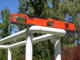
• An EM38 is an example of an electromagnetic induction (EMI) device which contains two coils of wire; one for creating a magnetic field (‘Transmitter coil’) and the other for sensing an external magnetic field (‘Receiver coil’).
• EMI devices work by rapidly modulating electric current in the Transmitter coil  which acts as an electromagnet and this produces a rapidly oscillating ‘Primary Magnetic Field’.
• This field penetrates down into the soil (and into any other nearby object) and induces “eddy currents” in the soil. The  eddy currents induce a response ‘Secondary’ magnetic field which is then detected by the receiver coil located at the other end of the device (usually 0.5 or 1 m away from the transmitter coil). The separation between the transmitter and receiver soils, known as the inter-coil spacing gives the device its characteristic spirit-level shape. Sometimes these devices are packed into plastic tubes, which gives some of them their ‘plumber pipe’ look. But basically they are of the same type of internal design.
• When the instrument is set to ‘Quadrature phase’ (or ‘Quad Phase’) the receiver coil on the instrument is tuned to measure the strength of the induced magnetic fields which is then converted to a measure of the Apparent Electrical Conductivity (ECa) in soil.
• It is important to ensure the instrument is set to ‘Quad Phase’ since the electromagnetic current is modulated, and the detector is set to look for magnetic field modulations that are out of phase with the device’s primary magnetic field. That way the very small return signal can be measured and separated from the very large primary field produced by the instrument itself.

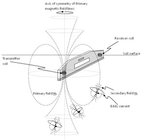Magnetic field orientation for an EM38-type device

• The volume of soil measured by an EMI sensor is governed by the physical penetration of the primary magnetic field into the soil and this is controlled by the orientation of the transmitter coil (ie the instrument) on top of the soil. Effectively the instrument can be thought of as a large bar magnet which can be orientated in either vertical dipole or horizontal dipole mode. In vertical dipole mode the magnetic field lines that induce the eddy current penetrate further into the soil.
• The strength of the primary magnetic field penetrating into the soil has a characteristic shape and this means the sensitivity of the instrument’s response to secondary magnetic fields (induced by the electrical conduction in the soil) also has a characteristic shape. In other words the depth sensitivity to the instrument has a particular shape and this is show below. In this graph the inter-coil spacing is 1 metre. If the inter-coil spacing changes then it is straight forward to work out the depth response curve. You simply scale it accordingly. A 0.5 m inter-coil spacing means you halve the values on the x-axis; a 2 m intercoil spacing means you     double them. The y-axis doesn’t change.

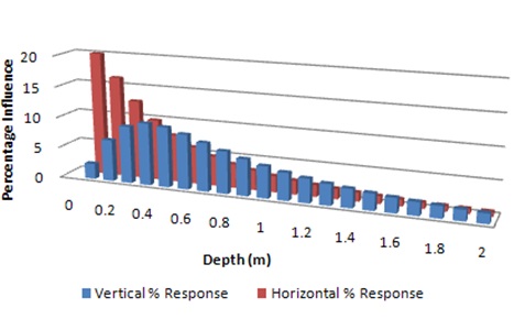
Sensitivity of EM38-type devices to soil water. salinity and texture at different depth below the soil surface. The blue bars indicate the response in vertical mode (most commonly used orientation) and the red bars are the horizontal orientation.

• The way you interpret the above graph is to think of it as a sensitivity curve. For example, when the instrument is orientated in horizontal dipole mode a certain electrical conductivity of the soil will elicit a great response in the instrument close to the surface that it would if the same conductivity were to exist deeper down. Similarly, when orientated in vertical dipole orientation, a high level of conductivity on or near the surface would have a smaller effect on the instrument than if it were to exist lower down- especially around the 40-50 cm depth mark. These response curves give rise to the notions of ‘response depth’- for an EM38 with 1 m inter-coil spacing, the horizontal dipole is considered to respond to about 50 cm depth and the vertical orientation to about 1.2 m depth or thereabouts. BUT, be aware that these are rough values based upon the notion that about 70-80% of the instruments total response is accumulated over this depth range. The fields, and hence the return signals can also emanate from much deeper down- especially if there are buried pipes (highly conductive) or a perched water table.

What Influences the strength of the return signal, and what do we get from an ECa survey?

• The factors, apart from proximity to either the transmitter or receiver coil, that influence the strength of the eddy current generated in the soil are; soil water content, soil ion content and soil clay content (which generally affects the former two anyway). Consider the combination of salinity (high ECe) and amount of water in the soil as a mutual amplification mechanism. If the soil is either wetter or contains more ions, you will get more current flowing in response to the primary field and hence a stronger return signal.
• Apart from salinity and waterlogging which can be detrimental to plant growth, most factors that drive high ECa response are associated with higher plant productivity eg. Increased clay content, CEC, organic matter, soil moisture and soil depth all increase ECa response. That’s why single ECa maps can often be useful for delineating basic differences in soil ‘types’ and why these can sometimes be used as the basis formulating prescription seed, irrigation and fertiliser maps. But remember, we are talking about relative measures here- ie one segment of soil appears different from the other. Be careful about assuming too much!
• It’s advised that single ECa surveys be performed when a soil is at field capacity as you need moisture in the soil to allow the current to flow.
• Field capacity is very difficult to define and even harder to achieve. Put it this way, the wetter a soil at the time of measurement the greater the range of response and hence greater potential ability to delineate differing soil zones in a paddock.
• Many one-off ECa surveys for delineating soil variability are often performed at soil moisture levels well below the refill point and this isn’t a major issue- just remember it may reduce the discrimination ability in terms of picking out areas of different soil characteristics.

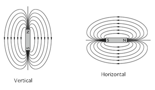Diagram showing the propagation of magnetic field from vertically  and a horizontally orientated bar magnet.

Can we measure the soil water content with an EM38?

• It appears that the answer is ‘yes’, although this is a cautious ‘yes’. At any given location in a field, over time the ECa will vary if the soil moisture distribution and ion content changes (let’s assume the soil type- eg clay etc doesn’t). Where there is relatively small leaching occurring over time (ie the ion content and distribution doesn’t change much), then the ECa changes over time can be dominated by the water content changes. And remember that it is the vertical distribution of water content that is at play here- and this can result from evapo—transpiration or simply horizontal and vertical drainage.
• Certainly in our own work we have found that, over time, the relationship between ECa -and neutron probe counts is linear for vertosol sites that are not confounded by high ECe or where there is not a significant jump in ion content at depth. Here we have determined the average soil moisture content over a depth range (eg 50 cm to 1.5 m for vertical orientation and surface to 50 cm for horizontal orientation).
• Assuming the linearity applies, these two ECa – neutron probe measurements taken at the same location can be used to infer the neutron probe count at that site for subsequent ECa measurements.
• There may not be a huge difference between the slopes of the linear relationships at various sites on uniform cracking clay soils. Remember, the gradient of an ECa versus soil moisture line is effectively the amplification effect of the water and ion content at work. Between soil zones and across landscapes we do expect significant variations in the ECa and soil moisture relationship.

How can we practically measure soil water with an EM38?

1. .Without calibration to actual soil moisture: Multiple surveys at various moisture levels, on the same transects or sites.
   - Use the highest and the lowest ECa measurements recorded as the “full” and “empty” bucket values for that site.
   - Each site will have its own “bucket size” and this will potentially change for crop species.
   - Calculate % full at any measurement time at any site – we know it’s approximately a straight line response.
   - This technique is useful for explaining unknown sources of variability in trials, but requires routine measurements throughout a cropping season.
2. With calibration to average actual soil moisture for the EM38 depth of response: Take a point ECa measurement of a wet soil, pull a core to determine the average VMC or mm’s of water then do the same at that site when it is drier.
   - This gives the actual ECa change for the depth of penetration of the EM38 and a corresponding soil moisture change.
   - Perform in multiple locations across a field to determine if the slope varies and use a single calibration across the field or individual calibrations for individual zones if necessary.
   - This calibrating can be performed retrospectively to determine actual soil moisture if the “without calibration” technique was previously used.

It can't be that easy...

• Geonics EMI devices require user calibration at the beginning of each use.
• The trick is to ensure that the instrument is responding the same way at the beginning of each survey in a multi-temporal set of measurements. The easiest way we have found to do this is to expose the instrument to a test coil (called a ‘Q-coil’) in isolation from the soil surface and record the response before each survey or sampling exercise.
• Geonics devices are generally robust and stable; with correct calibration you can minimise error over the extent of a growing season or subsequent growing seasons.
• The greater the soil moisture change between calibrating dates the better – you want a measure when the bucket is full and when it is empty to get the most accurate estimation of the gradient of ECa to VMC response.
• Revisit exactly the same spot when you take measurements from one day to the next. Peg them out if they’re within a plot or use a RTK guidance system to ensure the same transects are travelled for mapping.
• Recalibration of previous EM38 surveys, retrospectively, is not possible unless you know how the instrument was behaving back then and currently at the time of the calibrating cores.
• The EM38 seems to have a soccer ball sized response area directly under each coil, take cores from under one or both coils for calibration to soil moisture (1m apart). Removal of the 2” core doesn’t change the ECa response, so you can come back to the same site and take a subsequent core as close as possible, within reason.

Other important observations we’ve made:

• There is no easy way to calibrate an EMI device to compare water levels between two vastly different soil types. You must use a site specific calibration due to the way the instrument responds on each soil type if the slopes are too dissimilar.
• Measuring soil moisture with an EM38 in this manner is possible because during and between successive growing seasons three of the main factors that influence ECa remain relatively stable – soil clay content, soil depth and soil salinity (ECe). This is a big assumption unless it’s measured.
• It is hard to get a good correlation between gravimetric water or even standard volumetric water content and ECa¬ in cracking clay soils unless we account for the changes in the bulk density as water dependent swelling and contracting occurs in these soils. A formula to estimate bulk density of a cracking clay soil, adapted from Yule, 1984 is:
  Bulk Density = ((1-0.08)/(1/2.65+x))
  Where: x = gravimetric water (weight of water/weight of dry soil)
• VMC = (weight of water/density of water)/(weight of dry soil/Bulk Density)
• Proximity to metal objects is and the size of the metal object is important, if using aluminium neutron probe access tubes they need to be at least 0.5 m from either coil. Position the centre of the EM over the tube (risky) or both coils >1m away to be sure of no interference.

Useful References

Stanley, J.N., Lamb, D.W., Falzon, G. and Schneider, D.A. (2014) "Apparent electrical conductivity (ECa) as a surrogate for neutron probe counts to measure soil moisture content in heavy clay soils (Vertosols)". Soil Research, 52: 373–378

Stanley, J.N., Lamb, D.W., Irvine, S.E. and Schneider, D.A. (2014) "The effect of aluminum neutron probe access tubes on the apparent electrical conductivity recorded by an electromagnetic soil survey sensor" IEEE Geoscience and Remote Sensing Letters, 11 (1) 333-336 (DOI 10.1109/LGRS.2013.2257673).Yule, D.F. 1984. Volumetric calculations in cracking clay soils. In: Reviews in Rural Science: The Properties and Utilization of Cracking Clay Soils.